Revision Doc - Mid-Semester Exam

MATH1051

Revision

Chapter 2 - Vectors

2.1 Definition: Function, Domain, Range

Let $X$ and $Y$ be subsets of $\mathbb{R}$. A function $f:X\to Y$ is a rule which assigns to every element $x\in X$ exactly one element $f(x)\in Y$ called the value of $f$ at $x$. Here $X$ is called the domain of $f$ and

$$f(X)=\{f(x)\mid x\in X\}$$

is called the range of $f$, also written range$(f)$.

The range of $f$, $f(X)$, is a subset of $Y$. The range is the set of all possible values of $f(x)$ as $x$ varies throughout the domain. Note that $f(X)$ is not necessarily equal to all of $Y$.

Link to original

2.5 Exponential Functions

An exponential function is one of the form $f(x)=a^x$, where the base $a$ us a positive constant, and $x$ is said to be the exponent or power. One very common exponential function which we shall see often in this course is given by $f(x)=e^x$. It cuts the $y-$axis at $y=1.$

---
title: Exponential Function
xLabel: 
yLabel: 
bounds: [-10,10,-10,10]
disableZoom: true
grid: true
---
f(x)=2^x

Exponential functions are very useful for modelling many natural phenomena such as population growth (base $a>1$) and radioactive decay (base $0<a<1$).

Link to original

2.7 One-to-one Functions

A function $f:X\to Y$ is said to be one-to-one or injective if $\forall x_1,x_2\in X$.

On the graph of $f$, the 1-1 property holds exactly if any horizontal line $y=$ constant cuts through the curve in at most one place.

If one $x$ corresponds to another $x$, then it is not one-to-one. Similarly, if $y$ corresponds to another $y$ of the same value, then the function is not one-to-one.

2.7.1 Example

If the value of the function $y=x^2+3$:

---
title: 
xLabel: 
yLabel: 
bounds: [-10,10,-10,10]
disableZoom: false
grid: true
---
y=x^2+3

Then this is not a one-to-one function. This is because it does pass the vertical line test (with one $x$ corresponding to one $x$ only), but it does not pass the horizontal line test (for example, $x=2\cap x=-2$ yield the same $y$ value (with $y=7$)).

On the other hand, for example, $y=e^{2x}$:

---
title: 
xLabel: 
yLabel: 
bounds: [-10,10,-10,10]
disableZoom: false
grid: true
---
y=exp(2x)

Link to original

2.12 Inverse Trigonometric Functions

The function $y=\sin x$ is 1-1 if we just define it over the interval $\left[\frac{\pi }{2},\frac{\pi }{2}\right]$. The inverse function for this part of $\sin x$ is denoted $\arcsin x$. Thus $\arcsin x$ is defined on the interval $[-1,1]$ and takes values in the range $\left[-\frac{\pi }{2},\frac{\pi }{2}\right]$. The graph can easily be obtained by reflecting the graph of $\sin x$ about the line $y=x$ over the appropriate interval.

Similarly $y=\cos x$ is 1-1 on the interval $[0,\pi ]$ and its inverse function is denoted $\arccos x$. The function $\arccos x$ is defined on $[-1,1]$ and takes values in the range $[0,\pi ]$.

Also, $\tan$ is 1-1 on the open interval $\left(-\frac{\pi }{2},\frac{\pi }{2}\right)$ with inverse function denoted by $\arctan x$. Hence $\arctan$ has the domain $(-\infty ,\infty )$ with values in the range $\left(-\frac{\pi }{2},\frac{\pi }{2}\right)$.

---
title: 
xLabel: 
yLabel: 
bounds: [-10,10,-10,10]
disableZoom: false
grid: true
---
f^(-1)(x)=(exp(x)/(1+2*exp(x)))

Link to original

Chapter 3 - Sequences

3.1 Formal Definition: Sequence

More formally, a sequence is a function, with domain being $\{0,1,2,3,\dots \}$. We can also take the domain as $\{1,2,3,\dots \}$ and start the sequence at $a_1$ rather than $a_0$.

If $a:\{0,1,2,\dots \}\to \mathbb{R}$ is a function, viewed as a sequence, then we write $a_0$ instead of $a(0)$, $a_1$ instead of $a(1)$, etc.

Link to original

3.3 Limits

Let $\{a_n{\}}_{n=0}^{\infty }$ be a sequence. Then

$$\underset{n\to \infty }{\lim }{a}_n=\ell ,\ell \in \mathbb{R}$$

As $a_n$ approaches $\ell$, $n$ gets larger and larger. $a_n$ is always close to $\ell$ for $n$ sufficiently large.

3.3.1 Convention

If a sequence $\{a_n{\}}_{n=0}^{\infty }$ has limit $\ell \in \mathbb{R}$, we say that $a_n$ converges to $\ell$ and that the sequence $\{a_n{\}}_{n=0}^{\infty }$ is convergent. Otherwise the sequence is divergent.

Link to original

3.4 Theorem: Limit Laws

Caution

The following limit laws apply provided that the separate limits exist (that is $\{a_n\}$ and $\{b_n\}$ are convergent):

Suppose that $\{a_n\}$ and $\{b_n\}$ are convergent sequences such that

$$\underset{n\to \infty }{\lim }{a}_n=\ell \text{ and }\underset{n\to \infty }{\lim }{b}_n=m$$

and $c$ is a constant. Then

$$\begin{array}{rl}\underset{n\to \infty }{\lim }(a_n\pm b_n)& =\ell \pm m;\\ \underset{n\to \infty }{\lim }c{a}_n& =c\ell ;\\ \underset{n\to \infty }{\lim }(a_n{b}_n)& =\ell m;\\ \underset{n\to \infty }{\lim }\frac{a_n}{b_n}& =\frac{\ell }{m}\end{array}$$ Link to original

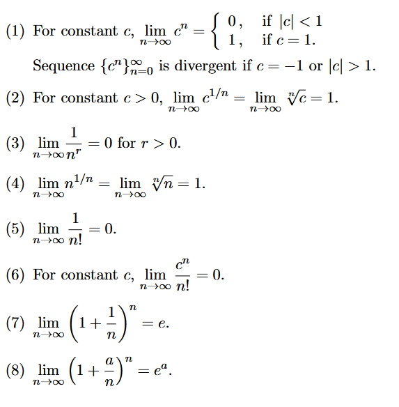
3.5 Useful Sequences to Remember

Take care with inequalities and limits. For example $\frac{1}{n}>0$ for all $n$ but ${\lim }_{n\to \infty }\frac{1}{n}=0$. In general, even if $a_n>b_n$ for all $n$, we can only conclude ${\lim }_{n\to \infty }{a}_n\ge {\lim }_{n\to \infty }{b}_n$. Note the $\ge$.

Link to original

3.6 Theorem: Squeeze

If $a_n\le b_n\le c_n$ for $n\ge n_0$ for some $n_0\in \mathbb{N}$ and ${\lim }_{n\to \infty }{a}_n={\lim }_{n\to \infty }{c}_n=\ell$, then

$$\underset{n\to \infty }{\lim }{b}_n=\ell$$

3.6.1 Example

Use the squeeze theorem on $\{a_n\}$, where $a_n=\frac{1}{n}\sin n$.

Since

$$-1\le \sin n\le 1,\text{ for }n\ge 1,$$

we have

$$-\frac{1}{n}\le a_n\le \frac{1}{n}$$

Now

$$\underset{n\to \infty }{\lim }-\frac{1}{n}=\underset{n\to \infty }{\lim }\frac{1}{n}=0$$ Link to original

Chapter 4 - Limits

4.1 Definition: Limit

(Stewart, p.50) Let $f(x)$ be a function and $\ell \in \mathbb{R}$. We say $f(x)$ approaches the limit $\ell$ (or converges to the limit $\ell$) as $x$ approaches $a$ if we can make the value of $f(x)$ arbitrarily close to $\ell$ (as close to $\ell$ as we like) by taking $x$ to be sufficiently close to $a$ but not equal to $a$.

We write

$$\underset{x\to a}{\lim }f(x)=\ell$$

Roughly speaking, $f(x)$ is close to $\ell$ for all $x$ values sufficiently close to $a$, with $x\ne a$. The limit “predicts” what should happen at $x=a$ by looking at $x$ values close to but not equal to $a$.

4.1.1 Some Basic Limits

$$\underset{x\to a}{\lim }1=1$$ $$\underset{x\to a}{\lim }x=a$$ Link to original

Transclude of Limits#42-properties

4.3 One-sided Limits

Consider the piecewise function

$$f(x)=\{\begin{array}{llc}& 1,& x\ge 0\\ & -2,& x<0\end{array}$$

Notice that $x{\lim }_{n\to \infty }f(x)=1$, but ${\lim }_{x\to 0,x<0}f(x)=-2$. Therefore, the limit as $x]\to 0$ does not exist. We can, however, talk about the one-sided limits.

In the above example, we say that the limit as $x\to 0$ from above (or from the right) equals 1 and we write

$$\underset{x\to 0^{+}}{\lim }f(x)=1$$

Similarly, we say that the limit as $x\to 0$ from below (or from the left) equals -2 and we write

$$\underset{x\to 0^{-}}{\lim }f(x)=-2$$

In general, for ${\lim }_{x\to a^{+}}f(x)=\ell ,$ just consider $x$ with $x>a$ and similarly for ${\lim }_{x\to a^{-}}f(x)=\ell$, consider only $x<a$.

Link to original

4.6 Some Important Limits

The following limits are fundamental. We omit the proofs. Combined with the properties given in 4.2 Properties and the Squeeze Principle in 4.4, these will enable you to compute a range of other limits.

$$\begin{array}{c}\underset{x\to 0}{\lim }\frac{\sin x}{x}=1\end{array}$$ $$\underset{x\to 0}{\lim }\frac{1-\cos x}{x^2}=\frac{1}{2}$$ $$\underset{x\to 0}{\lim }\frac{e^x-1}{x}=1$$

4.6.1 Precise Definition

Let $f$ be a function defined on some open interval that contains the number $a$, except possibly $a$ itself. The we write

$$\underset{x\to a}{\lim }f(x)=\ell$$

if for every number $ϵ>0$ there is a number $\delta >0$ such that

$$\mid f(x)-\ell \mid <ϵ\text{ whenever }0<\mid x-a\mid <\delta$$Link to original

Chapter 5 - Continuity

Transclude of Continuity#51-definition-of-continuity

Transclude of Continuity#52-continuity-of-intervals

Transclude of Continuity#54-the-intermediate-value-theorem-ivt

Chapter 6 - Derivatives

6.2 Definition of Derivative

The derivative of $f$ at $x$ is defined by

$$f^{\prime }(x)-\underset{h\to 0}{\lim }\frac{f(x+h)-f(x)}{h}$$

We say that $f$ is differentiable at some point $x$ if this limit exists. Further, we say that $f$ is differentiable on an open interval if it is differentiable at every point in the interval. Note that $f^{\prime }(a)$ is the slope of the tangent line to the graph of $y=f(x)$ at $x=a.$

We have thus defined a new function $f^{\prime }$, called the derivative of $f$. Sometimes we use the Leibniz notation $\frac{dy}{dx}$ or $\frac{df}{dx}$ in place of $f^{\prime }(x).$

Note that if $f$ is differentiable at $a$, there holds:

$$f^{\prime }(a)=\underset{x\to a}{\lim }\frac{f(x)-f(a)}{x-a}$$

6.2.1 Example

Using the definition of the derivative (“from first principles”), find the derivative of $f(x)=x^2+x$.

Using the definition for a derivative, we find:

$$\begin{array}{rl}{f}^{\prime }(x)& =\underset{h\to 0}{\lim }\frac{f(x+h)-f(x)}{h}\\ & =\underset{h\to 0}{\lim }\frac{(x+h{)}^2+(x+h)-(x^2+x)}{h}\\ & =\underset{h\to 0}{\lim }\frac{x^2+2xh+h^2+x+h-x^2-x}{h}\\ & =\underset{h\to 0}{\lim }\frac{2xh+h^2+h}{h}\\ & =\underset{h\to 0}{\lim }(2x+h+1)\\ & =2x+1\end{array}$$ Link to original

6.5 Derivative of an Inverse Function

Suppose $y=f^{-1}(x)$, where $f^{-1}$ is the inverse of $f$. To obtain $\frac{dy}{dx}$ we use

$$x=f(f^{-1}(x))=f(y)$$

Differentiating both sides with respect to $x$ using the chain rule gives:

$$\begin{array}{rl}1& =\frac{d}{dx}(x)\\ & =\frac{d}{dx}f(y)\\ & =\frac{df}{dy}\times \frac{dy}{dx}\\ & =\frac{dx}{dy}\times \frac{dy}{dx}\end{array}$$

Hence, if $\frac{dx}{dy}\ne 0:$

$$\frac{dy}{dx}=\frac{1}{\left(\frac{dx}{dy}\right)}$$ Link to original

6.6 L’Hopital’s Rule

Suppose that $f$ and $g$ are differentiable and $g^{\prime }(x)\ne 0$ near $a$ (except possibly at $a$). Suppose that

$$\underset{x\to a}{\lim }f(x)=0\text{ and }\underset{x\to a}{\lim }g(x)=0$$

or

$$\underset{x\to a}{\lim }f(x)=\pm \infty \text{ and }\underset{x\to a}{\lim }g(x)=\pm \infty$$

then

$$\underset{x\to a}{\lim }\frac{f(x)}{g(x)}=\underset{x\to a}{\lim }\frac{f^{\prime }(x)}{g^{\prime }(x)}$$

if the limit on the right exists or is $\pm \infty$.

6.6.1 Example

Find ${\lim }_{x\to 1}\frac{\ln x}{x-1}$.

Note that

$$\underset{x\to 1}{\lim }\ln x=\underset{x\to 1}{\lim }(x-1)=0$$

Hence, we cannot use

$$\underset{x\to 0}{\lim }\frac{f(x)}{g(x)}=\frac{{\lim }_{x\to 0}f(x)}{{\lim }_{x\to 0}g(x)}$$

Instead, we use L’Hopital’s rule to get:

$$\underset{x\to 1}{\lim }\frac{\ln x}{x-1}=\underset{x\to 1}{\lim }\frac{\frac{1}{x}}{1}$$

if this limit exits,

$$=1.$$ Link to original

6.7 Continuous Extension of Sequences

Sometimes L’Hopital’s rule can be used to evaluate limits of sequences. Let $f$ be a function on the real numbers such that ${\lim }_{x\to \infty }f(x)$ exists. Let $f(n)=a_n$ for natural numbers $n$. Then:

$$\underset{n\to \infty }{\lim }{a}_n=\underset{x\to \infty }{\lim }f(x)$$

6.7.1 Example

Evaluate ${\lim }_{n\to \infty }\frac{\ln x}{n}$.

Define $f(x)=\frac{\ln x}{x}$. Hence

$$\begin{array}{rl}\underset{x\to \infty }{\lim }f(x)& =\underset{x\to \infty }{\lim }\frac{\ln x}{x}\\ & =\underset{x\to \infty }{\lim }\frac{1/x}{1}\text{ by L’Hopital’s rule}\\ & ⟹\underset{n\to \infty }{\lim }\frac{\ln n}{n}=0\end{array}$$ Link to original

6.8 The Mean Value Theorem (MVT)

Let $f$ be continuous on $[a,b]$ and differentiable on $(a,b)$. Then

$$\frac{f(b)-f(a)}{b-a}=f^{\prime }(c)$$

for some $c$, where $a<c<b$.

Note $f^{\prime }(c)$ is the slope of $y=f(x)$ at $x=c$ and $\frac{f(b)-f(a)}{b-a}$ is the slope of the chord joining $A=(a,f(a))$ to $B=(b,f(b))$.

Link to original

6.9 Increasing/Decreasing Test

Suppose that $f$ is continuous on $[a,b]$ and differentiable on $(a,b)$.

8.4 Critical Points and Curve Sketching

A function $f$ has a global maximum at $c$ if $f(c)\ge f(x)$ for all $x$ in the domain of $f$. The number $f(c)$ is called the maximum value of $f$ on its domain. A global maximum is also called an absolute maximum.

A function $f$ has a global minimum at $c$ if if $f(c)\le f(x)$ for all $x$ in the domain of $f$. The number $f(c)$ is called the minimum value of $f$ on its domain. A global minimum is also called an absolute minimum.

A function $f$ has a local maximum at $c$ if $f(c)\ge f(x)$ for all $x$ near $c$.

A function $f$ has a local minimum at $c$ if $f(c)\le f(x)$ for all $x$ near $c$.

If $f$ has a local maximum or minimum at $a$, and if $f^{\prime }(a)$ exists, then $f^{\prime }(a)=0$. The point $(a,f(a))$ is a critical point of the function $f$ if $f^{\prime }(a)=0$ or if $f^{\prime }(a)$ does not exists (but $f(a)$ does).

Thus, all local maxima and minima are critical points. Note however, that not all critical points are local maxima or minima.

To find any local maximum or minimum of a function $f$, we solve the equation $f^{\prime }=0$. We can then classify any critical points we find using the information about the function near the critical point.

A function $f$ is strictly increasing on an interval $[a,b]$ if for all $x_1$ and $x_2$ in $[a,b],f(x_1)<f(x_2)$ whenever $x_1<x_2$.

If $f^{\prime }(x)>0$ on an interval, then $f$ is strictly increasing on that interval. If $f^{\prime }(x)<0$ on an interval, then $f$ is strictly decreasing on that interval. If $f^{\prime }(x)=0$ on an interval, then $f$ is constant on that interval.

First Derivative Test

Suppose that the function $f$ has a critical point at $x=c$. Then

If $f^{\prime }$ changes sign from positive to negative at $c$, then $f$ has a local maximum at $c$. If $f^{\prime }$ changes sign from negative to positive at $c$, then $f$ has a local minimum at $c$. If $f^{\prime }$ does not change sign at $c$, then $f$ has neither a local maximum nor a local minimum at $c$.

The Second Derivative

The second derivative of a function $f$ is the derivative of the derived function $f^{\prime }$. The second derivative of $f$ is denoted $f"$.

The second derivative provides information about the concavity of the graph of a function.

If the graph of $f$ lies above all of its tangent lines on an interval, then it is concave up on that interval. If the graph of $f$ lies below all of its tangent lines on an interval, then it is concave down on that interval.

If $f"(x)>0$ for all $x$ in an interval, then the graph of $f$ is concave up on that interval. If $f"(x)<0$ for all $x$ in an interval, then the graph of $f$ is concave down on that interval.

Second Derivative Test

Suppose $f"$ is a continuous function near a point $c$.

If $f^{\prime }(c)=0$ and $f"(c)>0$, then $f$ has a local minimum (concave up) at $c$. If $f^{\prime }(c)=0$ and $f"(c)<0$, then $f$ has a local maximum (concave down) at $c$. If $f"(c)=0$, then this test is inconclusive.

Curve Sketching

To sketch the curve of a function $y=f(x)$:

• Determine the domain of $f$.
• Determine the $y$-intercept of the graph by evaluating $f(0)$.
• If it is possible to solve the equation $f(x)=0$, find the $x$-intercepts of the graph.
• Determine $f^{\prime }$ and identify the intervals of which $f$ is increasing and the intervals on which $f$ is decreasing.
• Find the critical points of $f$. Determine which critical points are local maxima or local minima (use first or second derivative test).
• Determine $f"$ and identify the intervals on which $f$ is concave up and the intervals on which $f$ is concave down.
• Sketch the graph.

Link to original

Link to original