Ordinary Differential Equations

MATH1052

Contents

Just Some Basic Information To Know:

Rough Course Outline:

• Chapter 1 - Ordinary differential equations
• Chapter 2 - Functions of several variables
• Chapter 3 - Partial Derivatives and Tangent Planes
• Chapter 4 - Max and min Problems on surfaces
• Chapter 5 - Parameterisation of curves and line integrals

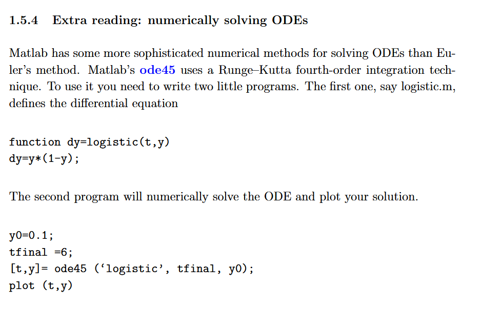
Introductory Comments on Lectures on ODE’s

Ordinary Differential Equations (ODEs)

An ODE is an equation containing a function $y$ of a single independent variable $x$, as well as derivatives of the function. An equation of the form

$$f\left(x,y,\frac{dy}{dx},\frac{d^{2}y}{d{x}^2},\dots ,\frac{d^{n}y}{d{x}^n}\right)=0$$

is called an ODE of order $n$. Here $f$ encodes a relationship between $x$ and $y$ and some of its derivatives.

title: Solutions
collapse: open
 
A *solution* of an ODE is a function $y(x)$ that satisfies the ODE for all $x$ in some (real) domain.
 
A solution	 to an $n$-th order [[2024/Definitions/ODE|ODE]] contains up to $n$ arbitrary constants.

Initial Value Problem (IVP)

An IVP is the problem of finding a solution of a differential equation that satisfies one or more initial conditions.

Imposing initial conditions will usually fix (some of) the arbitrary constants appearing in the general solution to the differential equation.

Common Notation

$$y^{\prime }=\frac{dy}{dx},y^{\prime \prime }=\frac{d^{2}y}{dx},y^{(k)}=\frac{d^{k}y}{d{x}^k},k\in \mathbb{N}$$

This allows us to write a first order ODE in the form

$$y^{\prime }=g(x,y)$$

---

1 Ordinary Differential Equations

1.1 Introduction

There are two types of DE’s:

• Ordinary Differential Equations (ODE), where the unknown function is a function of only one variable
• Partial Differential Equations (PDE), where the unknown function is a function of more than one variable. We will not consider PDEs in this course.

1.1.1 Examples of ODEs

• Unbounded population growth: $P^{\prime }(t)$ = $kP$
• Bounded population growth: $P^{\prime }(t)$ = $kP(1-P/\theta )$
• Motion due to gravity: $m{y}^{\prime \prime }(t)$ = $-mg$
• Spring system: $m{x}^{\prime \prime }(t)$ = $-kx$

title: Reminder
collapse: open
Derivatives such as $x'(t)$ and $x''(t)$ with respect to time are often written as $\dot{x}$ and $\ddot{x}$ respectively.
 

1.1.3 Solution to an ODE

Suppose that we are given an ODE for $y$ which is an unknown function of $x$. then $y=f(x)$ is said to be a solution to the ODE if the ODE is satisfied when $y=f(x)$ and its Derivatives are substituted into the equation.

Example

Show that $y=y(x)=A\exp (x^2/2)$ is a solution to the ODE $y^{\prime }=xy$.

$$\text{We need to show that }y=A\exp (x^2/2)\text{ satisfies the ODE.}$$ $$\begin{array}{rl}\text{Calculate LHS}& \\ y^{\prime }& =\frac{d}{dx}\left(A\exp x^2/2\right)\\ & =Ax\exp x^2/2=xy\\ & \therefore \text{ RHS as required}\end{array}$$

When asked to solve an ODE, you are expected to find all possible solutions.

Solving ODE of various forms. For an ODE that involves only the unknown function $y$ and its first Derivatives, the general solution will involve one arbitrary constant.

Example

Find the general solution to the differential equation $y^{\prime }=x^2$.

$$\frac{dy}{dx}=x^2⟹y=\int x^{2}dx=\frac{x^3}{3}+c$$

This is the general solution for this ODE.

1.1.4 Initial Value Problems

An Initial Value Problem (IVP) is the problem of solving an ODE subject to some initial conditions of the form $y(t_0)=a,y^{\prime }(t_0)=b$, etc.

The solution to an initial value problem no longer contains arbitrary constants from the general solution to the ODE - these are determined by the initial conditions.

Example

Question

A flow-meter in a pipeline measures flow-through as $2+\sin t$ litres/second. How much fluid passes through the pipeline from time zero up to time $T$?

Success

As Flow-through time is volume/unit time, the general solution would be $\frac{dv}{dt}=2+\sin t⟹v(t)=2t-\cos t+c$ $v(0)=2{\times }_0-\cos 0+c=c-1=0⟹c=1$ and that means $v(T)=2T-\cos T+1$

1.1.5 The order of an ODE

The highest order Derivatives in an ODE defines the order of the ODE.

That would mean that first derivative, e.g. $\dot{x}$ would have a higher order of the ODE than $\ddot{x}$ and so on.

1.1.6 Riding Your Bike at Constant Speed

Find the position of your bike (at time $t$) if you are travelling at a constant speed of 60km/h along a perfectly straight road.

If $x=x(t)$ is the distance you have travelled at time $t$ then the corresponding ODE is

$$\frac{dx}{dt}=60.$$

This yields the general solution to the ODE

$$x(t)=60t+C$$

To determine the constant $C$ we need more info, such as the initial position at time 0, in which that would be IVP.

For different vales of $C$ we get different solutions, and below we graph some of these. If $C=0$ then $y=60t$. All the other solutions are parallel to this line.

The curves $y=60t+C$ are called solution curves to the ODE ($\ast$). Note that in this particular case all curves are straight lines with slope 60.

1.1.7 Motion of Projectiles

In this case, we can consider finding an expression for gravity.

Example

Question

Consider an apple falling under gravity. Find an expression for the height $y$ of the apple at time $t$.

Newton’s 2nd law of motion is $F=ma$. The velocity of the apple is $\dot{y}$, and the acceleration of the apple would be $\ddot{y}$.

The force exerted on the apple is $F=-mg$.

$$⟹F=-mg=\ddot{m}y$$ $$⟹\ddot{y}=-g$$

Integrating this, $\dot{y}=-gt+c$ and $y=-\frac{g{t}^2}{2}+ct+d$

1.1.8 Extra Reading: Realistic Models

For realistic objects, a projectile motion includes air resistance.

Most moving objects of a good model deal with air resistance proportional to the square of the velocity: $\frac{d^{2}y}{d{t}^2}=-g-f\frac{dy}{dt}\left|\frac{dy}{dt}\right|$ For slower objects, a good model has air resistance proportional to velocity:

Realistic models may also include the fact that gravity diminishes as you move away from the earth’s surface (Newton’s inverse square law).

Example

Consider the motion of a ball subject to air resistance proportional to the square of the speed. Note that the air resistance vector is always directed against the direction of motion.

Decompose the coordinates to $x$ and $y$ directions and again apply Newton’s 2nd law of motion.

Note that

$$\sin \theta =\frac{\dot{y}}{\sqrt{{\dot{x}}^2+{\dot{y}}^2}}\text{and }\cos \theta =\frac{\dot{x}}{\sqrt{{\dot{x}}^2+{\dot{y}}^2}}$$

Hence $F=ma$ in the $y$ directions gives

$$\begin{array}{rl}& m\ddot{y}=-mg-F_D\sin \theta \\ & \Rightarrow m\ddot{y}=-mg-k{v}^2\sin \theta \\ & \Rightarrow m\ddot{y}=-mg-k({\dot{x}}^2+{\dot{y}}^2)\times \frac{\dot{y}}{\sqrt{{\dot{x}}^2+{\dot{y}}^2}}\\ & \Rightarrow \ddot{y}=-g-\frac{k}{m}\dot{y}\sqrt{{\dot{x}}^2+{\dot{y}}^2}\end{array}$$

In much of the same way:

$$\ddot{x}=-\frac{k}{m}\dot{x}\sqrt{{\dot{x}}^2+{\dot{y}}^2}$$

This is a coupled system of ODE which is extremely difficult to solve analytically. However, numerical solutions are easy to obtain.

1.1.9 Analytical and Numerical Solutions

To solve an ODE (or IVP) analytically means to give a solution curve in terms of continuous functions defined over a specific interval, where the solution is obtained exactly by analytic means (e.g., by integration). The solutions satisfies the ODE (and initial conditions) on direct substitution.

To solve an ODE or IVP numerically means to use an algorithm to generate a sequence of points which approximates a solution curve.

title: Important Remark
collapse: open
 
As we have already seen, the ODE
$$
\frac{dy}{dt}=f(t)
$$ 
can be solved analytically. The *solution* simply is 
 
$$
y=\int f(t) \, dt 
$$
 

1.2 Slope Fields and Equilibrium Solutions

In order to solve $\frac{dy}{dt}=f(t)$, we need to integrate. If we do this for a more general first-order ODE, this would not work. An example would be like this:

$$\frac{dy}{dt}=f(t,y)$$

Either way, we note that at $(t,y)=(a,b)$ the slope of $y(t)$ is $f(a,b)$. So what one can do is as follows:

title: Ways to Solve General Form ODEs
 
- In the $ty$-plane, at $(t,y) = (a,b)$, draw a small straight line with slope $f(a,b)$.
- Repeat the process for many different values of $(a,b)$.
- The resulting diagram is called the *slope field.*

Note

The slope field can be generated without having to solve the ODE.

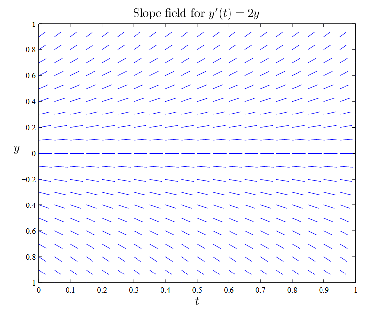
From the slope field of $y^{\prime }(t)=2y$, we can see that $y=0$ is one of the solution curves. It is a constant or Equilibrium Solution.

1.2.3 Stability of Equilibrium Solutions

From a slope field, you can decide whether an equilibrium solution is stable or not by determining if solution curves will tend toward the equilibrium solution or away as time increases.

Formally, an equilibrium solution $y(t)=y_0$ to the differential equation $y^{\prime }=f(t,y)$ is stable if the initial value problem:

$$\frac{dy}{dt}=f(t,y),y(0)=y_0\pm ϵ$$

has a solution $y(t)$ that satisfies

$$\underset{t\to \infty }{\lim }y(t)=y_0$$

In other words, if you start sufficiently close to a stable Equilibrium Solution, then you will approach that equilibrium solution.

Important Remark

It is an important point that equilibrium solutions cannot be crossed by other solution curves. In fact, no solutions curves can cross each other because this would mean that in some point(s) $y^{\prime }(t)$ has more than one value. Equilibrium solutions therefore partition the solution space.

1.2.5 Main Points

Main Points

• You should understand how to generate and interpret slope fields.
• You should understand what is meant by an equilibrium solution and how to find one.
• You should be able to determine the stability of an equilibrium solution.
• You should understand that uniqueness of solutions to an IVP implies that solutions cannot cross.

---

---

1.3 Euler’s Method for Solving ODEs Numerically

Euler’s Method uses tangent lines as approximations to solution curves. The tangent line to a solution curve of $y^{\prime }=f(t,y)$ at $(t_0,y_0)$ is

$$y=y_0+f(t_0,y_0)(t-t_0).$$

This approximates the curve when $t$ is close to $t_0$.

Using $\nabla t$ as the step size for our algorithm, let

$$t_1=t_0+\nabla t,t_2=t_1+\nabla t,t_3=t_2+\nabla t,\dots ,t_n=t_{n-1}+\nabla t$$

To find approximate $y$ values at these times, use the following equations in sequence:

$$y_1=y_0+f(t_0,y_0)\nabla t$$

and so on.

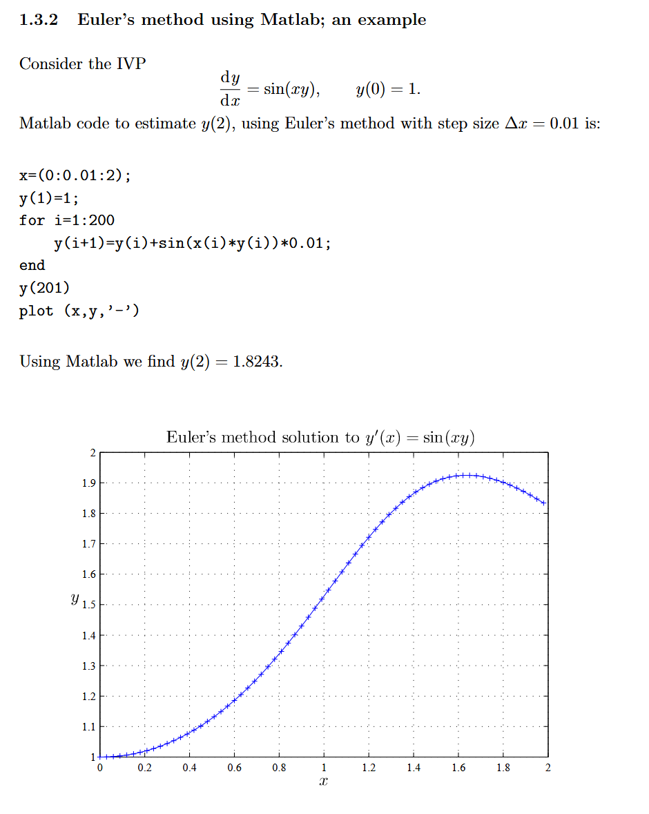
1.3.2 Euler’s Method Using Matlab; an Example

1.3.4 Main Points

Main Points

• You should understand how slope fields lead to Euler’s Method
• You should know how to approximate a solution to an IVP using Euler’s Method by hand.
• You should know how to implement Euler’s Method in Matlab.
• You should understand that errors can be a problem in the approximate solution, especially if a large step size is used.

1.4 Separable ODEs

Caution

It is very important that you become skilled at identifying and solving this type of ODE.

1.4.1 Definition

A first-order ODE is called separable if it can be written in the form

$$\frac{dy}{dx}=f(x)g(y).$$

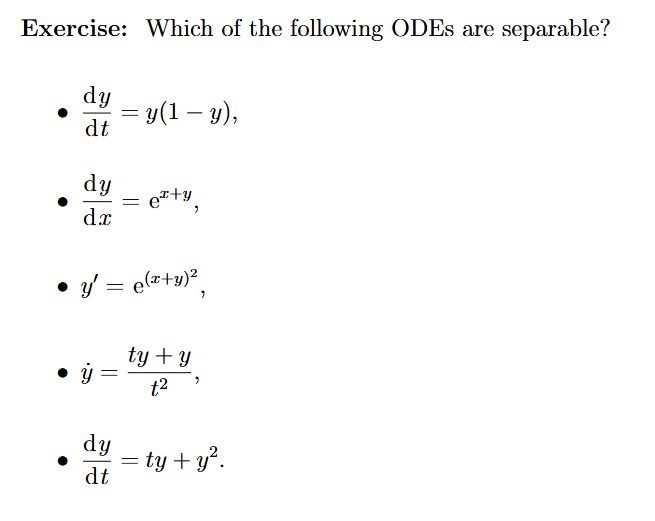
Answer

1st one, 4th one and 5th one.

1.4.2 Solving Separable ODEs

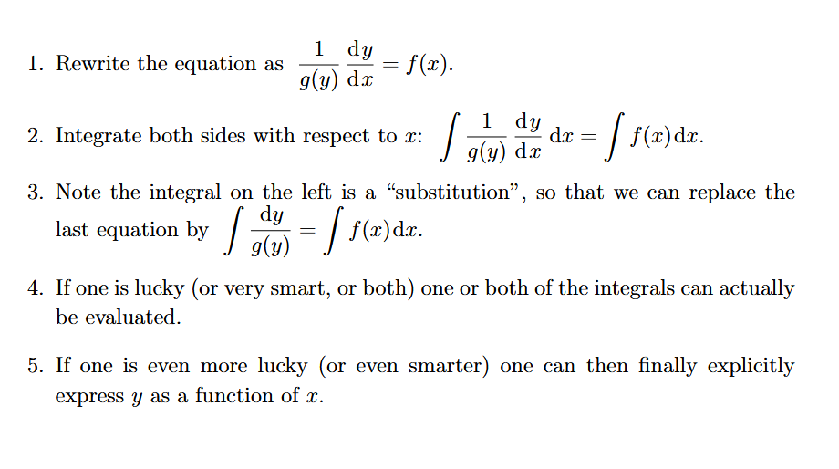
Attention

The last two steps are not always possible. Just try and simplify as best you can :D

1.4.3 Singular Solutions

For solving separable ODEs we always try and start by rewriting the equation as $\frac{1}{g(y)}\frac{dy}{dx}=f(x)$. Since we cannot divide by zero, this means that our method is only valid provided that $g(y)\ne 0$.

If there is such a case such as $\mathbf{a}$ such that $g(\mathbf{a})=0$ then the ODE will have the Equilibrium Solution $y(x)=a$.

1.4.4 Main Points

Main Points

• You should be able to identify a first-order separable ODE.
• You should know how to solve a separable ODE.
• You should understand that equilibrium and singular solutions are equivalent and must be checked for when solving a separable ODE.

1.5 Applications: Law of Cooling, Population Growth

1.5.1 Newton’s Law of Cooling

Newton’s Law of Cooling states that the rate at which a “body” cools is proportional to the temperature difference between the body and its surrounding medium.

If $T$ is the temperature of the body and $T_m$ the temperature of the surrounding medium, then according to Newton,

$$\frac{dT}{dt}=-k(T-T_m),k>0$$

Here is the constant $k$ is chosen such that if $T>T_m,T^{\prime }(t)$ is negative, describing cooling.

1.5.4 Extra Reading

1.5.5 Main Points

Main Points

• You should be able to apply Newton’s Law of Cooling and solving the resulting IVP.
• You should know how to model population growth and solve the resulting IVP.
• You should be able to interpret the obtained solutions.

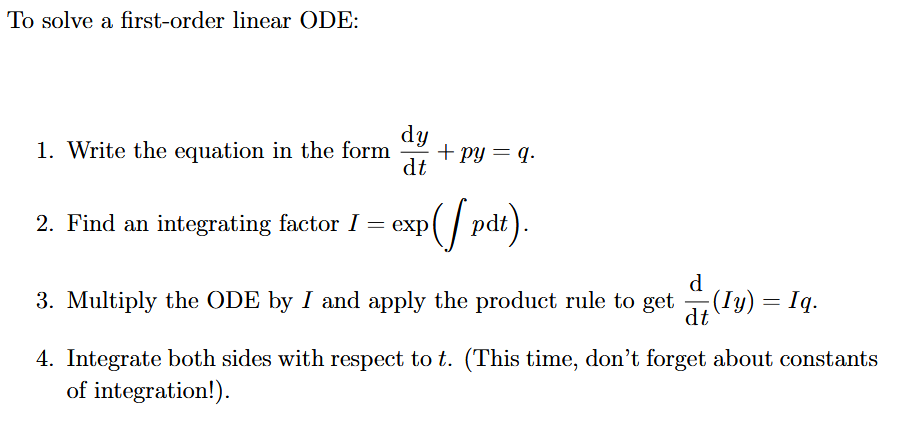
1.6 Solving Linear First Order Equations

Method

If you cannot solve a differential equation by separation, your next plan of attack should be to test if it is linear and use the integration factor method described below.

1.6.1 Definition

A first-order is linear if it can be put into the form

$$\frac{dy}{dt}+p(t)y=q(t)$$

for some functions $p(t)$ and $q(t)$.

Note

Recall the product rule for differentiation. This formula is key to solving first-order linear ODEs.

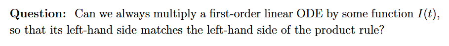
We can do something called an Integrating Factor.

Given the ODE

$$\frac{dy}{dt}+p(t)y=q(t)$$

we multiply by the yet-to-be-found integrating factor $I(t)$:

$$I(t)\frac{dy}{dt}+I(t)p(t)y=I(t)q(t)$$

We think of $I$ as $g$ and $y$ as $f$. Then the left term on the left is $f^{\prime }g$ and the second term on the left to be $f{g}^{\prime }=y{I}^{\prime }$. Given that the second term is $Ipy$, we infer that $I$ must satisfy the ODE

$$I^{\prime }(t)=I(t)p(t)$$

This is good news since this is a separable ODE which we already know how to solve:

$$I(t)=\exp \left(\int p(t)dt\right)$$

Summary

1.6.3 Main Points

Main Points

• You need to be able to identify a first-order ODE.
• You need to be able to solve a first-order linear ODE using an Integrating Factor.

1.7 Linear Second-Order Differential Equations with Constant Coefficients